Abstract
Quantifying an organic light-emitting diode (OLED) requires more than recording maximum external quantum efficiency (EQE) or a narrow electroluminescence (EL) peak. The measurement must connect calibrated spectral radiant flux, photon counting, charge injection, angular emission and human-vision-weighted photometry without silently changing definitions. This mechanism- and metrology-first guide explains how EQE, luminance, current efficiency, luminous efficacy, spectral FWHM, CIE chromaticity, efficiency roll-off and operational lifetime should be acquired and compared. It distinguishes direct measurements from optical assumptions, model-derived metrics and cross-paper inferences, with illustrative diagrams rather than unverified source plots. Particular attention is given to non-Lambertian devices, wavelength-response-corrected relative spectra for chromaticity, J90-based roll-off, and the distinction between laboratory-pixel luminance ageing and lighting-panel flux-maintenance statistics. The document is an educational scientific review, not a new measurement standard or an experimental report.
Learning objectives
Derive the photon/electron EQE definition; identify when normal-direction measurements bias EQE; separate radiometric and photometric quantities; compute chromaticity from an appropriately corrected relative radiant-power spectrum and specified standard observer; read EQE–J and EQE–L curves; define LT95/LT50 under actual electrical stress; and construct a falsifiable device-comparison audit.
1. Define the object and measurement boundary before the metric
A molecular emitter, a neat or doped photoluminescent film, a laboratory single-pixel OLED, an integrated tandem OLED and a commercially driven display panel are different objects. Their spectra, extraction pathways, electrical inputs and spatial uniformity cannot be conflated. For a bottom-emitting research pixel, report substrate, emitting aperture or overlap area, layer stack and thicknesses, top/bottom emission direction, active area used for current density, emission side(s), encapsulation and test atmosphere. Record whether measurements were acquired before, during or after burn-in. [1, 4, 11]
EQE per injected electron is especially sensitive to the electrical and optical accounting convention. A tandem stack can generate photons from multiple emissive units per injected pair, while a quoted “internal quantum efficiency” is ordinarily inferred using an optical model rather than collected directly. Different organic families (fluorescence, phosphorescence, TADF, MR-TADF and hyperfluorescence) use distinct triplet-harvesting mechanisms, yet the external measurement must obey the same dimensional rules. Nominal current density is J = I/A_e, with the effective area A_e explicitly stated; leakage and nonuniform current spreading may invalidate naive geometric conversion. [1, 6, 7]
2. Calibrated spectral photon accounting and angular collection
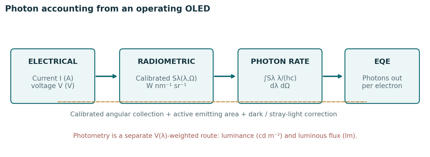
Let Sλ(λ,Ω) be the spectral radiant intensity leaving the selected device-side collection hemisphere in W sr⁻¹ nm⁻¹, measured after background subtraction and wavelength-dependent instrument calibration. Then photon emission rate is Ṅph = ∫Ω ∫λ Sλ(λ,Ω)·λ/(hc) dλ dΩ, provided units are consistent and the optical geometry covers the defined solid angle. The injected electron rate is Ṅe = I/e, giving EQE = Ṅph/Ṅe. This form assumes a single electrical current through the defined device and must not double-count flux leaving both sides. If the measured quantity is spectral radiance L_e,λ (W m⁻² sr⁻¹ nm⁻¹) instead, first integrate L_e,λ cosθ over the visible emitting area to obtain spectral radiant intensity, before integrating over wavelength and solid angle. Uniform area, azimuthal symmetry and emission from only one device side are assumptions to validate or disclose, not automatic properties of an OLED. [1, 12]
A calibrated integrating sphere can capture substantial angular flux but requires consideration of self-absorption, port geometry, detector spectral responsivity, stray illumination and the emitting side(s) actually sampled. Angle-resolved EL records wavelength- and angle-dependent signals and integrates the actual radiation pattern; polarization, azimuth and collection geometry may also matter. Assuming a Lambertian profile from forward luminance alone is not generally defensible. In their device examples Archer and colleagues demonstrated deviations large enough to materially affect EQE, especially for microcavity/top-emitting structures. This is a reason to measure the angular profile, not a universal fixed percentage correction. [1]
2.1 Dimensional worked example (hypothetical)
For a monochromatic 500 nm photon, Eγ ≈ hc/λ ≈ 3.97 × 10⁻¹⁹ J. If independently integrated total outward radiant power were 0.25 mW and current were 1.00 mA, photon rate would be ≈ 6.29 × 10¹⁴ s⁻¹ and electron rate ≈ 6.24 × 10¹⁵ s⁻¹, yielding EQE ≈ 10.1%. This hypothetical result assumes the 0.25 mW already covers the stated angular/side collection boundary; one forward detector reading cannot replace the integral.
2.2 Practical measurement workflow and uncertainty checks
For a traceable research-pixel EQE, acquire dark-corrected detector counts and current at a defined, stabilized drive point; apply wavelength and spectral-responsivity calibration and the documented detector-geometry conversion to obtain spectral radiant intensity (W sr⁻¹ nm⁻¹) or another explicitly identified radiometric quantity; document the detector aperture, collection solid angle and emitting-area geometry; measure or independently validate the angular/azimuth distribution (and declare any assumed azimuthal symmetry); integrate photon energy weighting over wavelength and the agreed collection sides; then divide the outward photon rate by I/e. Repeat at several drive levels while monitoring spectral shifts and temporal drift. A radiance-based input must first be integrated over projected emitting area and angles; a spectral radiant-intensity input must not be multiplied by emitting area again. Uncertainty should include responsivity, angular coverage, alignment, effective area, current and stability. [1, 12]
3. Photometric and radiometric metrics are not interchangeable
Photometric weighting represents a standard observer’s visual response, not photon probability. The photopic luminous flux is Φv = 683 lm W⁻¹ × ∫ Φe,λ(λ)V(λ)dλ, where Φe,λ is spectral radiant flux and V(λ) is the agreed luminous-efficiency function. Luminance L (cd m⁻²) describes directional luminous intensity per projected emitting area; luminous flux Φv is in lumens. Current efficiency ηC = Iv/I (cd A⁻¹) uses luminous intensity under a specified viewing direction, while luminous efficacy ηP = Φv/(U I) (lm W⁻¹), with U the measured device voltage, uses total emitted luminous flux and electrical power; neither is identical to EQE. [5]
Two blue spectra with equal photon EQE need not have equal luminance because V(λ) changes strongly with wavelength. Conversion of cd A⁻¹ to EQE using only a peak wavelength or an assumed Lambertian distribution can hide systematic error. Record the full calibrated EL spectrum and angular convention. If a work reports ηout or EQE ≈ γ·Φint,eff·ηout, identify the photon-generation boundary and whether extraction and dipole-orientation inputs came from an optical simulation; avoid multiplying a triplet-harvesting factor twice. [1, 5]
| Metric | Definition / unit | Do not assume |
|---|---|---|
| EQE | Outward photon rate / injected electron rate (%) | Equals PLQY or cd A⁻¹ |
| Radiant flux | Angle-integrated emitted optical power (W) | Equals forward power-meter reading |
| Luminance | Directional photometric output (cd m⁻²) | Equals luminous flux (lm) |
| Current efficiency | Luminous intensity / current (cd A⁻¹) | Comparable across spectra without context |
| Luminous efficacy | Total luminous flux / VI (lm W⁻¹) | Same as optical power efficiency |
| EQE@specified drive | EQE at stated J or luminance | Equals EQEmax |
Table 1. Device-efficiency quantities, units and common invalid substitutions.
4. Spectral acquisition and the wavelength–energy convention
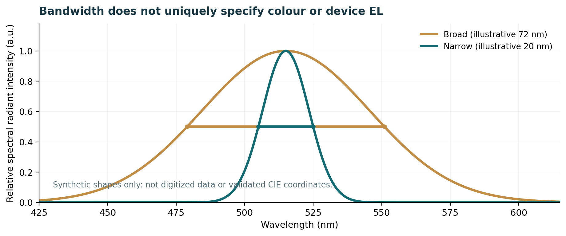
A device EL spectrum needs stated excitation mode (electrical, not PL), wavelength interval and spectrometer resolution, intensity calibration, source angular acceptance, drive point, ambient conditions and background subtraction. Report peak wavelength and FWHM with units, together with complete line shape where possible; a reported FWHM can depend on the instrument line-spread function, overlapping bands and fitting or interpolation choices. The optical cavity can narrow or reshape the angular EL without changing the isolated molecule’s vibronic potential-energy surfaces. [1, 2]
Spectral density transforms under E = hc/λ: I_E(E) = I_λ(λ)|dλ/dE| = I_λ(λ)λ²/(hc), evaluated at λ = hc/E. For a sufficiently narrow band, ΔE ≈ (hc/λ₀²)Δλ is a local-width approximation only. A full density transformation can shift the numerical peak and FWHM; no universal “nm-to-eV FWHM” conversion is exact for arbitrary line shapes. The relevant spectral quantity must also be specified: radiant-power density and photon-count density each have their own weighting.
5. Colorimetry, colour purity and viewing-angle stability
For a specified CIE standard observer, use a wavelength-calibrated, detector-response-corrected relative spectral radiant-power distribution P(λ) to compute X ∝ ∫P(λ)x̄(λ)dλ, Y ∝ ∫P(λ)ȳ(λ)dλ and Z ∝ ∫P(λ)z̄(λ)dλ with consistent sampling. Absolute radiant-power calibration is not needed for chromaticity alone: multiplication of P(λ) by any wavelength-independent positive factor leaves x and y unchanged. However, a wavelength-dependent detector bias distorts the spectral shape and cannot be removed by simply normalizing its maximum. CIE 1931 chromaticities are x = X/(X+Y+Z), y = Y/(X+Y+Z); CIE 1976 coordinates are u′ = 4X/(X+15Y+3Z), v′ = 9Y/(X+15Y+3Z). The common proportionality factor cancels for chromaticity. A photon-count spectrum Nλ(λ) per wavelength must first be converted to the corresponding radiant-power spectral density through the photon energy hc/λ; numerical integration should document sampling/interpolation and the chosen observer. State 2° versus 10° observer, viewing geometry and electrical drive. [2, 3]
Narrow FWHM can help colour saturation but is not a sufficient measure of “color purity”: central wavelength, shoulders, residual sensitizer emission, optical microcavity, host/device environment and angular spectral shift also matter. Display gamut coverage is a multi-primary, system-level property and cannot be assigned to a single monochrome OLED pixel from its FWHM alone. Δu′v′ can be useful for documented angular drift or ageing but is not a universal perceptually uniform difference metric. Chromaticity may use a response-corrected relative SPD; neither an absolute radiometric flux calibration nor an arbitrary intensity scale is required. Avoid using a screenshot, poorly digitized plot or uncorrected detector spectrum as though it were a spectrally trustworthy distribution. [2, 4]
| Reported item | Minimum context | Unsupported shortcut |
|---|---|---|
| EL FWHM (nm/eV) | EL domain, resolution, wavelength axis, drive and angle | Identify terminal-molecule intrinsic width |
| CIE x,y or u′,v′ | Response-corrected relative SPD, observer and angle | Requires absolute power; or derive from peak alone |
| Angular color shift | Spectra at defined angles / azimuths | Assume normal view represents all angles |
| Color gamut | Declared multi-primary set and gamut reference | Claim display coverage from one single-color pixel |
| White-light rendering | SPD, CCT and chosen rendering metric | Treat as comparable to single-color saturation |
Table 2. Spectral and chromaticity reporting boundaries.
6. Efficiency roll-off: specify both the ordinate and the drive variable
Efficiency roll-off is a decrease in device EQE as current density and often luminance increase, but the physical interpretation depends on current balance, recombination-zone width, exciton density, molecular kinetics, field dependence, self-heating and measurement history. At minimum publish the raw or sufficiently sampled J–V–L data and EQE–J/EQE–L curves with active area, spectral/angular correction, bias sweep direction and temperature. EQEmax, EQE at 100 cd m⁻² and at 1000 cd m⁻², or a chosen application-specific current density are complementary rather than interchangeable metrics. [6, 8]
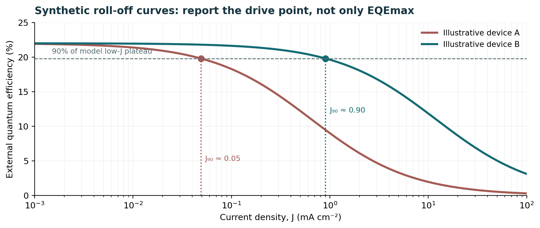
Diesing et al. defined J90 as the post-peak current density at which the EQE falls to 90% of the device’s peak EQE. Their literature analysis found that, even within kRISC ≈ (8–15) × 10⁵ s⁻¹, reported J90 values span approximately 0.03–40 mA cm⁻² (over three orders of magnitude); this is a within-study comparison across different devices, not a controlled molecular intervention. Neither kRISC nor ΔEST alone predicts practical TADF roll-off. If data never fall to 90% within the measurement range, report “J90 not reached” (with the range), rather than extrapolating an invented value. A J90 value is also conditional on the peak definition, noise/smoothing, wavelength-angular acquisition and electrical protocol. Report whether the post-peak 90% crossing was measured directly or obtained by interpolation between measured points; a plateau, noisy local maximum or incomplete drive range can make the threshold non-unique. [7]
7. Mechanistic diagnosis of roll-off: falsify alternatives
Candidate loss pathways include triplet–triplet annihilation (TTA), triplet–polaron quenching, singlet–triplet annihilation, field-induced quenching, changes in charge balance, recombination-zone localization, and nonuniform joule heating. Different emissive systems weigh these channels differently. For instance, Erickson and co-workers directly studied the role of recombination-zone width and bimolecular losses in distinct phosphorescent OLED architectures; one should not transfer the dominant channel or fitted coefficient into a TADF or HF device without reproducing its excitation environment. [6, 8]
Delayed PL, transient EL, impedance, single-carrier devices, carrier-selective layers, excitation-fluence tests and spatial/angle-dependent EL are complementary. A single EQE–J curve does not identify a unique microscopic annihilation constant. When using an effective triplet density T (cm⁻³) and polaron density p (cm⁻³), an illustrative depletion law dT/dt = G − k₁T − 2kTTA T² − kTPQ Tp makes the order of candidate terms explicit, but uniform-density assumptions and the factor-two event convention must be reported. Fit uncertainties and alternative kinetic models are essential before causal claims.
| Observed change | Possible mechanisms | Independent test |
|---|---|---|
| Steep EQE–J decline | TTA/TPQ/STA; charge imbalance | Fluence PL + transient EL + single-carrier controls |
| Angle/EL spectrum varies with J | Cavity/recombination-zone shift | Angle-resolved EL at matched J |
| Voltage rises during sweep | Electrical/thermal ageing; trapping | Reverse sweep, thermal/time stabilization |
| Delayed emission changes | Spin conversion and multiple losses | Temperature/fluence-dependent film + EL data |
| Low J90, high EQEmax | High-brightness bottleneck | EQE at stated practical luminance + J90 |
Table 3. Roll-off hypotheses and discriminating evidence.
8. Operational lifetime: endpoints are protocols, not intrinsic constants
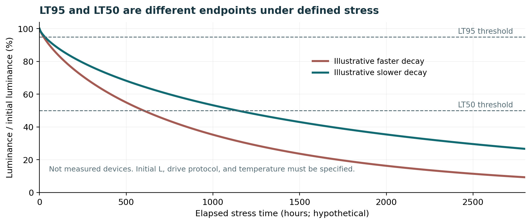
LT95 is the elapsed time at which luminance drops to 95% of the specified initial luminance L0; LT50 is the analogous 50% endpoint. L0 should be defined at a stated reference time after any documented stabilization or burn-in. Each endpoint must be attached to a defined device, stress environment and drive mode. A constant-current ageing run often yields a falling luminance and rising voltage; a constant-luminance controller instead changes current/voltage to maintain a brightness set point, so its “lifetime” requires a distinct failure criterion (such as required current, voltage, efficiency or inability to hold set point). Under closed-loop constant-luminance operation, an unchanged controlled L(t) cannot yield conventional luminance-crossing LT95/LT50 until the controller fails or its set point is changed. These are not automatically interchangeable tests. [9, 11]
Report at least L0, LT endpoint, whether measured or extrapolated, drive waveform/duty cycle, constant-current or constant-luminance mode, temperature, humidity/encapsulation, active area, pixel/sample count, failure rule, calibration checks and any burn-in/preconditioning. Also report color shift and voltage evolution where relevant. Reversible transient quenching (including self-heating) does not by itself establish irreversible exciton-driven chemical degradation. Different chemical ageing mechanisms can be coupled to carrier balance, long-lived excitations, bond stability, morphological changes and interfaces. [9, 10]
9. Accelerated ageing is a model and must be validated
A commonly used empirical acceleration relation, written with an explicit reference rather than a dimensionful bare power, is LT_x(L0) = LT_x(Lref)·(Lref/L0)^n. Here x is the defined decay endpoint, Lref is a measured reference initial luminance and n is a fitted acceleration exponent; the relation is only a same-protocol empirical hypothesis that must be tested across multiple initial luminances. Neither n = 1.5 nor n = 1.8 is a universal physical constant. A reported LT50 extrapolated from short tests may be fragile if different stresses activate different degradation pathways, thermal effects, electrode issues or charge accumulation. Whenever possible, include model diagnostics, uncertainty bounds and a measured-data window that visibly supports the extrapolation. [10, 11]
The IEC 62922:2016/AMD1:2021 general-lighting amendment provides lifetime-estimation information for OLED panels, including cautions about the absence of one universal degradation model. The amendment’s informative Annex H concerns OLED general-lighting panels, including luminous-flux maintenance and estimation of median useful life across a product population. Such panel-oriented flux-maintenance statistics cannot be equated automatically to the luminance-derived LT95 or LT50 of a single constant-current laboratory pixel. The analogy is methodological only; it does not certify any research diode to the licensed IEC document. Likewise, IEC 62341-6-1:2025 is a display-measurement standard with its own scope, not a universal laboratory SOP for every organic emitter experiment. [4, 11]
10. Primary studies as a measurement-quality casebook
Archer et al. [1] separate current–voltage–luminance measurements from angle-resolved spectral output, exposing device-specific errors in a forward-direction Lambertian shortcut. The lesson is to measure rather than borrow an angular correction. Cusumano and colleagues [12] offer a photodiode-based alternative: their simple total-power calculation uses a Lambertian spatial-emission assumption with a suitably positioned detector, with extension to non-Lambertian sources requiring an independently measured spatial pattern. Their measured diode signal also requires an emission-spectrum-dependent responsivity correction. Neither technique removes the need to state calibration, collection geometry and uncertainty.
Diesing et al. [7] show why a benchmark must record an operating curve: their J90 analysis reports over three orders of magnitude in J90 among published TADF devices with comparable kRISC, whereas an EQEmax-only table conceals the practical roll-off problem. This is a database-level correlation and does not establish the rate-limiting mechanism for a specific OLED. Murawski et al. [6] and Erickson et al. [8] frame TTA/TPQ and recombination-zone dynamics as testable alternatives, not causes to be inferred from EQE alone. Stability reviews [9, 10] provide background mechanisms but cannot be treated as independent experiments reproducing every quoted lifetime. No numerical cross-paper leaderboard is presented here because optical calibration, test stress, stack and unit count are not harmonized.
11. Minimum device data package and uncertainty ledger
A reproducible measurement package comprises (a) full stack and emitting-area metadata; (b) raw I–V–L measurements with sweep timing, direction, compliance limits and device heating checks; (c) calibrated angular and spectral radiant intensity with detector response, dark correction and geometry; (d) derived EQE–J/EQE–L, cd A⁻¹ and lm W⁻¹ with calculation code, formulas and uncertainty; (e) EL spectra and chromaticity by viewing angle; and (f) device ageing traces, stress protocol and replicate statistics. Publishing executable analysis scripts and machine-readable tables can make an efficiency claim independently reproducible even when exact device recipes remain restricted. [1, 4]
Build an uncertainty budget rather than quoting excessive digits. Typical contributors include detector calibration, spectral responsivity, sample alignment, aperture/angular integration, emission nonuniformity, stray light, effective electrical area, current meter calibration, wavelength calibration, temperature drift and device-to-device variability. Correlated calibration errors cannot simply be averaged away by repeated acquisitions. When only publisher abstracts or graphical plots are accessible, clearly mark numeric claims as provisional and avoid unsupported confidence intervals.
| Domain | Required values / provenance | Failure if missing |
|---|---|---|
| Identity / architecture | Host, guests, EML fraction, full stack, unit count, active area | Mix single-unit with tandem or film data |
| Calibration / geometry | Radiometer/spectrometer calibration, angular range, collection side | Hidden EQE collection bias |
| Electrical / photometric | J–V–L, EQE–J, EQE–L, cd/A, lm/W, protocols | Peak performance mistaken for operating value |
| Spectral / colorimetric | Response-corrected relative SPD, FWHM, observer, angle | Confusing normalized with response-corrected spectra |
| Time / statistics | Pixel luminance LTxx vs panel flux Lx; stress and replicate count | Single-pixel LT treated as panel median life |
| Inference / models | Optical fit, rate model, parameter uncertainties, exclusions | Model outputs mistaken for direct measurement |
Table 4. Minimum metadata for comparison and publication approval.
12. Falsifiable next steps and publication boundary
The most decisive research extension is a paired study of otherwise matched OLED stacks with systematically varied emissive-layer position, thickness, host/guest loading or optical cavity. Measure angle-resolved spectral radiance, normal luminance, current and temperature on the same stabilized pixels, then recompute EQE using both the directly observed angular distribution and a declared Lambertian approximation. The signed difference provides a testable, device-specific optical correction. Independently map EQE–J and EQE–L while tracking EL spectral shifts and active-area inhomogeneity. [1, 7]
For lifetime comparisons, stress replicate pixels at several L0 values with both temperature and current protocol documented; compare measured LT95 and LT50 within one protocol before fitting a bounded acceleration law. A mechanistic claim requires a prospective diagnostic (e.g., transient EL, chemical product signature, optical cavity change) that can discriminate reversible losses from cumulative ageing. Publish both positive and negative controls. The equations, figure captions, standard scope, reference-level audit and disclosed assumptions in this Expert Revised v3 educational guide were accepted by the scientific owner for public publication on 28 October 2026. This authorization does not certify uninspected standards or original data and does not substitute for separate website-build and deployment verification.
References and source-access status
- [1] Archer et al. (2021). Accurate Efficiency Measurements of Organic Light-Emitting Diodes via Angle-Resolved Spectroscopy. Advanced Optical Materials. https://doi.org/10.1002/adom.202000838
- [2] CIE 015:2018. Colorimetry, 4th Edition. Commission Internationale de l’Éclairage. https://doi.org/10.25039/TR.015.2018
- [3] CIE (2019). CIE 1931 colour-matching functions, 2° observer, 1 nm data set. https://doi.org/10.25039/CIE.DS.xvudnb9b
- [4] IEC 62341-6-1:2025. OLED displays – Part 6-1: Measuring methods of optical and electro-optical parameters. https://webstore.iec.ch/en/publication/85934
- [5] NIST. Realization of the candela (photopic weighting and K_m ≈ 683 lm W⁻¹). https://www.nist.gov/pml/sensor-science/optical-radiation/realization-candela
- [6] Murawski, Leo & Gather (2013). Efficiency Roll-Off in Organic Light-Emitting Diodes. Advanced Materials 25, 6801–6827. https://doi.org/10.1002/adma.201301603
- [7] Diesing et al. (2024). A figure of merit for efficiency roll-off in TADF-based organic LEDs. Nature 627, 747–753. https://doi.org/10.1038/s41586-024-07149-x
- [8] Erickson & Holmes (2014). Engineering Efficiency Roll-Off in Organic Light-Emitting Devices. Advanced Functional Materials. https://doi.org/10.1002/adfm.201401009
- [9] Swayamprabha et al. (2021; online 2020). Approaches for Long Lifetime Organic Light Emitting Diodes. Advanced Science 8, 2002254 (2021; online 2020). https://doi.org/10.1002/advs.202002254
- [10] Tankelevičiūtė, Samuel & Zysman-Colman (2024). The Blue Problem: OLED Stability and Degradation Mechanisms. Journal of Physical Chemistry Letters. https://doi.org/10.1021/acs.jpclett.3c03317
- [11] IEC 62922:2016/AMD1:2021. Organic light emitting diode (OLED) panels for general lighting – Performance requirements, Amendment 1. https://webstore.iec.ch/en/publication/62708
- [12] Cusumano et al. (2022). A simple method for the photometric characterization of organic light-emitting diodes. Solid-State Electronics 195, 108394 (2022). https://doi.org/10.1016/j.sse.2022.108394
Evidence disclosure
This revised, internally reviewed educational draft relies on official CIE/IEC/NIST descriptions, accessible research articles and article abstracts. Full licensed IEC/CIE standards, all journal Supporting Information, raw calibration logs and numerical re-analysis of each literature device have not been obtained or independently audited. Figures 1–4 are original, synthetic explanatory graphics; they are not reproduced source figures, measured data or device simulations. Claims about a named study retain the measurement/reporting boundary documented in the accompanying Source-to-Claim Audit. No external peer review, new experiment, exhaustive original-data verification or full licensed standards audit is asserted. Editorial acceptance and deployment verification are distinct records.